The math and the hacking
Michael Mulet - February 5th, 2023
The best way to show you what I did, and why, will be to jump into the code (which you can download here). The "meat" of this game in written in python and using the pytorch library. The code is then compiled for the web using the onnx runtime for the web.
Compressed Sensing
Compressed sensing is a method of acquiring data from a signal and reconstructing the signal. What makes it interesting is that the amount of measurements you make (m) is much less than the number of elements in the signal (n).
I'm not going to go into the theory of why it works, because I could find a lot of good resources on the internet:
- Video Lecture MIT 6.854 Spring 2016 Lecture 22: Compressed Sensing
- Lecture NotesCompressed Sensing and Sparse Recovery
- Book Compressed Sensing and its application
However, I did have trouble finding some good examples of how to implement it, so that's what I want to share here. Below you will be able to find the instructions on how to implement everything from wavelet transform to autodiff by hand.
Let's start by taking a measurement:
import torch
from torch import Tensor
def compressed_sensing(
    # Measurement Matrix is an m x n matrix
    measurement_matrix: Tensor,
    # signal is an n dimensional vector
    signal: Tensor):

    return torch.matmul(
                  measurement_matrix,
                  signal)

measurement = compressed_sensing(
                  measurement_matrix,
                  signal)
There, we sensed it! It's that easy. It's just matrix multiplication. Let's break it down.
# our signal
from PIL import Image
from torchvision.transforms.functional import pil_to_tensor

def get_signal():
  # this a 32x32 black and white image
  img = Image.open("images/1.png")
  signal = pil_to_tensor(img).flatten()
  return signal
The signal is just a bunch of pixels, in our case a 32x32 image that we flatten down to a 1024 dimensional vector.
The measurement matrix is a bit more complicated. There are a lot of choices you can make,
many of which depend on the signal being sensed. In all cases, the measurement matrix is a
matrix with dimensions m x n, where m is the number of measurements, and n is the
dimension of the signal (1024 in our case).
So what did I pick for the measurement matrix? I picked a random matrix from a bernoulli distribution. It has been shown that (with high probability) this matrix will be able to recover the signal. Plus, it's only a couple lines of code to generate.
import torch
def generate_bernoulli_measurement_matrix(
  measurements: int,
  signal_length: int) -> torch.Tensor:
    one =  torch.bernoulli(
           torch.empty(
                measurements,
                signal_length)
           .uniform_(0, 1))
    two = one - 1
    return one + two
There are structured matrices (faster to compute, and smaller to store), but I won't go into that here.
To recap, we take the signal and multiply it by the measurement matrix (random -1, and 1). What we get in return is a vector of measurement.
Sparsity and Wavelets
The entire point of compressed sensing is to recover the signal from the measurements. In the general sense, you can't just do this with any matrix. Because the number of measurements is less than the dimension of the signal, there are an infinite number of signals that could have generated the measurements. It's an underdetermined system.
We need to add some constraints to the problem. This is where the magic happens. The constraint we add is that the signal must be sparse. This means that the signal has a lot of zeros, See:
import torch
this_is_sparse = torch.tensor([
    0, 1, 0, 0, 0, 1, 0, 0, 1, 0,0])

# these number were chosen randomly
this_is_not_sparse = torch.tensor([
    81.694, 32.424, 22.22,50.55, 39.883, 99.10])
At this point, you might be thinking:
"Are images sparse?"
No, but we can transform the image to make it sparse. I've read before that natural images are sparse in the wavelet domain (A Mathematical Introduction to Compressive Sensing, Foucart, and Rauhut, page 11). A lot of people will probably be familiar with the fourier transform, but not everyone is familiar with the wavelet transform, so have a look below at a 2d wavelet transform of an image.
Fun Fact: Electrical engineers have to do a fourier transform every day. Otherwise their bodies will disintegrate into the sinusoids that make up everything.
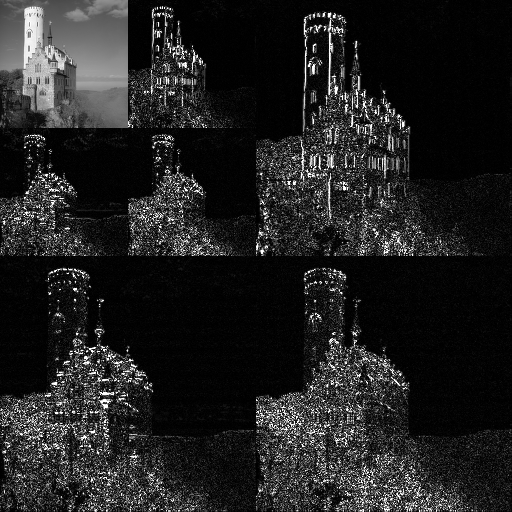
Look at how sparse this is! (Alessio Damato CC BY-SA 3.0 via Wikimedia Commons )
Specifically, I'm using the haar wavelet, the oldest and simplest wavelet. I mostly like to use it for low-resolution images because more complicated wavelets tend to have a "smoothing" effect that I find undesirable.
The haar wavelet is simple and computes in O(n) (faster than cooley-tukey's O(n log n)). I'm going to show how you compute it by using a 2d signal and 2d kernels.
Feel free to skip this, you would want to use torch.conv2d or a good library like PyTorch Wavelets Toolbox if you were doing this for real.
# manually convolving a 2d signal with
# 4 2d kernels to show how the
# haar wavelet works.
# We are using mutltiresolution analysis here
# which means we are going to do this a bunch of times, given by the level
# ( we apply the transformation again to the output of convolving the image
# the the lowpass kernel)
# Then we are going to do the inverse transformation
level = 2

power_of_2 = int(math.pow(2,level))
test_vector = torch.arange(0,power_of_2*power_of_2, dtype=torch.float).reshape((power_of_2,power_of_2))


#These are the coefficients of the haar wavelet
lowpass_kernel = 0.5* torch.tensor([[1,1],[1,1]], dtype=torch.float)
low_high_kernel = 0.5* torch.tensor([[1,1],[-1,-1]], dtype=torch.float)
high_low_kernel = 0.5* torch.tensor([[1,-1],[1,-1]], dtype=torch.float)
high_high_kernel = 0.5* torch.tensor([[1,-1],[-1,1]], dtype=torch.float)

def convolve_2d(d: int, kernel: torch.Tensor, mat: torch.Tensor):
    out = torch.zeros((d//2,d//2), dtype=torch.float)
    for row in range(0,d, 2):
        for col in range(0,d,2):
            out[row//2,col//2] = torch.mul(kernel, mat[row:row+2,col:col+2]).sum()
    return out

ll = test_vector
d = power_of_2
my_coefs = []
#This is the multiresolution analysis part
for _ in range(level):
    new_ll = convolve_2d(d, lowpass_kernel, ll)
    lh = convolve_2d(d, low_high_kernel, ll)
    hl = convolve_2d(d, high_low_kernel, ll)
    hh = convolve_2d(d, high_high_kernel, ll)
    my_coefs.append(torch.stack([lh,hl,hh]))
    ll = new_ll
    d = d//2
my_coefs.reverse()

#This big happy matrix will be the like the image above.
one_big_happy_matrix = torch.vstack([torch.hstack([ll,my_coefs[0][0]]),torch.hstack([my_coefs[0][1],my_coefs[0][2]])])
for i in range(1,level):
    one_big_happy_matrix = torch.vstack([torch.hstack([one_big_happy_matrix,my_coefs[i][0]]),torch.hstack([my_coefs[i][1],my_coefs[i][2]])])

# Now lets do the inverse transform
def convolve_2d_inverse(d: int, kernels: list[torch.Tensor], mat: torch.Tensor):
    # start with d is 2 by 2
    out = torch.zeros((d,d), dtype=torch.float)
    small_d = d//2
    for row in range(0,small_d):
        for col in range(0,small_d):
            for kernel_index,kernel in enumerate(kernels):
                out[row*2 + (1 if kernel_index >= 2 else 0) , col*2 + (1 if (kernel_index % 2) == 1 else 0)] = \
                kernel[0,0]*mat[row,col] + \
                kernel[0,1]*mat[row,col+small_d] + \
                kernel[1,0]*mat[row+small_d,col] + \
                kernel[1,1]*mat[row+small_d,col+small_d]
    for row in range(0, d):
        for col in range(0, d):
            mat[row,col] = out[row,col]

maybe_original = one_big_happy_matrix.clone()
d = 2
for i in range(level):
    convolve_2d_inverse(d, [lowpass_kernel, low_high_kernel, high_low_kernel, high_high_kernel], maybe_original)
    d = d*2
Now that you know how to do the wavelet transform, I'm going to put the wavelet transform into an orthogonal matrix. This will make the derivative easier to derive, which I do in a later step. It's probably the slowest method of computing a wavelet transform
transform_matrix, inverse_transform_matrix = generate_wavelet_transform(2)
This returns two matrices, the first is the wavelet transform matrix, and the second is the inverse wavelet transform matrix. Also worth noting, since the matrix is an orthogonal matrix, the inverse is just the transpose.
Reconstruction
Now we can begin the reconstruction. Again, there are multiple ways to do this, but I'm going to use the basis pursuit denoising because it works well and is really easy:
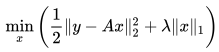
Put into words, we want to find the value for x that minimizes the mean squared error between the measurements and the signal while at the the same time minimizing the l1 norm of x (the l1 norm is just the sum of the absolute values of x). Minimizing the l1 norm is our way of saying we want to find the sparsest solution to the problem.
In the above equation, y is the measurements, and A is the measurement matrix multiplied by the inverse transform matrix, and lambda is just a constant.
Note: Quick aside about A, and x.
x starts out as just random noise:
x = torch.randn(signal.shape)
We want x to be in the wavelet domain (because our image is sparse in the wavelet domain). So, we have to take the inverse wavelet transform to move x into the image domain.
x_in_image_domain = torch.matmul(
                inverse_transform,
                x)
Then we can do the measurements using the measurement matrix.
measurement_of_x = torch.matmul(
              measurement_matrix,
              x_in_image_domain)
Because matrix multiplication is associative, we can combine the last two steps to get our A matrix.
A = torch.matmul(measurement_matrix, inverse_transform)
Now, we can put it all together to get our loss function.
# start with a random x. It's just noise, so it doesn't matter what it is.
x = torch.randn(signal.shape)
A = torch.matmul(measurement_matrix, inverse_transform)
loss = 0.5*torch.square(
  measurement - torch.matmul(A,x)
  ).sum()
  + lambda*torch.abs(x).sum()
Basis pursuit denoising is a convex quadratic problem, so we don't have to worry about local minima. We can choose any optimization method we want. I'm going to use stochastic gradient descent because it's easy to implement. First, we'll implement it using pytorch, using the same methods we would use for training a neural network:
import torch

# First we do some sensing
true_signal = get_signal()
measurement_matrix = generate_bernoulli_measurement_matrix(row: 768, columns: 1024)
measurement = compressed_sensing(measurement_matrix, true_signal)

# Now we reconstruct the signal
_transform, inverse_transform = generate_wavelet_transform(true_signal.shape)

# start with a random x. It's just noise, so it doesn't matter what it is.
x = torch.randn(true_signal.shape[1], requires_grad=True)
A = torch.matmul(measurement_matrix, inverse_transform)

optimizer = torch.optim.SGD([x], lr=0.0003, momentum=0.9)
lambda = 10_000
for i in range(50):
    optimizer.zero_grad()
    # same loss as before
    loss = 0.5*torch.square(
          measurement - torch.matmul(A,x)
        ).sum() \
      + lambda*torch.abs(x).sum()
    loss.backward()
    optimizer.step()
# done!
# x is now a lossy approximation of the true signal
I will note that I found the lambda, the learning rate, the momentum, and the number of iterations by trial and error.
In case you unfamiliar with pytorch:
- the
requires_grad=Trueis what tells pytorch to keep track of the gradient of x. - The
optimizer.zero_grad()is what tells pytorch to reset the gradient of x to 0. - The
loss.backward()is what tells pytorch to compute the gradient of x using pytorch's autodiff - The
optimizer.step()is what tells pytorch to update x using the gradient of x and the learning rate.
Now, because basic pursuit denoising is so simple, I'm going to do the autodiff by hand to show what is actually happening. It's actually only a few lines of code:
x = torch.randn(true_signal.shape[1])

for i in range(50):
  measurement_of_x = torch.matmul(A, x)
  difference = measurement_of_x - measurement
  d_weights_1 = 10_000*torch.sign(x)
  d_weights_2 = torch.matmul(A.t(), difference)
  diffs = d_weights_1 + d_weights_2

  # doing SGD with momentum of 0.9
  diffs += 0.9 * previous_diffs
  previous_diffs = diffs
  # then we update the weights using a learning rate of 0.0003
  reconstruction -= 0.0003 * diffs
Let's go over why this works. First, let's look at the loss function:
loss = 0.5*torch.square(difference).sum() + lambda*torch.abs(x).sum()
You'll notice that we don't actually compute this.
That's because the actual value of the loss function doesn't matter. It's the gradient of the loss function with respect to x that matters.
So, let's calculate the gradient. We'll start by taking the derivative of lambda*torch.abs(x).sum(). We are going to use the chain rule to calculate the derivative of the loss function by finding the derivative of each individual part, and then multiplying them together
Note: Let z be a free variable that I'm making up to show how to do the derivative of each part. We will substitute z for our current gradient as we go along
- start with a derivative of 1
- derivative of lambda*z is lambda (because lambda is a constant)
- derivative of the sum (ie. z_1 + z_2 .... z) with respect to z is 1,
- derivative of abs(z) is sign(z)
let's bring it together with the chain rule
derivative of lambda*abs(z).sum is 1*lambda * sign(z)
Then plug in x into z and 10_000 into lambda and we get
d_weights_1 = 10_000*torch.sign(x)
Now let's look at:
0.5*torch.square(difference).sum()
- similar to above we start with 1.
- derivative of 0.5 * z with respect to z is 0.5
- derivative of z^2 with respect to z is 2*z
- derivative of the sum ( z_1 + z_2 ... z) is 1
Multiply together to get
1*0.5 * 2 * z = z
Because of the chain rule, we will plug in the variable difference for z
So our gradient so far is:
difference * (derivative of difference with respect to x)
So, let's calculate the derivative of difference with respect to x. Recall that difference is:
difference = measurement_of_x - measurement
As I said before, the derivative of adding and subtracting a constant is just 1. Our new gradient is:
difference * (derivative measurement_of_x with respect to x)
Now, let's calculate the derivative of measurement_of_x with respect to x. Recall that measurement_of_x is:
measurement_of_x = torch.matmul(A, x)
The derivative of a matrix A multiplied z with respect to z is
the transpose of A multiplied by z. Let's plugin difference, and get our the last part
of this gradient:
torch.matmul(A.t(), difference)
So our final gradient is:
10_000*torch.sign(x) + torch.matmul(A.t(), difference)
And now you know how to do basic pursuit denoising by hand. That's it for the math, now for the hacking!
The hacking
This entire project started because I was hacking around with compressed sensing, seeing how I could corrupt the measurements and still recover the signal. I actually found that I can reduce the entire reconstruction to noise just by flipping about 8 bits (I do cheat a little bit, by converting from float32 to int16, but you can verify that the loss of precision is not the problem)
See how it works (in typescript this time. ort is the onnx runtime):
const corrupt_samples = (samples: ort.Tensor) => {
  for(let i = 0; i < 8; i++){
    samples.data[i] &= 0x7fff;
  }
}
What this does is set the most significant bit of the first 8 samples to 0. The samples are most likely represented as two's complement integers, so this will have one of two effects:
- If the sample is positive, this will have no effect.
- If the sample is negative, this will make it positive and will most likely increase the magnitude of the sample. Doing this will corrupt basically any reconstructed image into noise.
Now, I don't consider this to be novel (obviously taking some samples and multiplying by an extremely large number will corrupt the reconstruction), but I do think it's fun because it corrupts the whole image by changing the minimal number of bits.
The game
So here is how the game works, I take your input from the "terminal" and assign a value to it. I am not a fan of how riddles often have multiple correct answers, so to make the answers more sparse, I eliminated 10 letters of the alphabet (if you look closely you'll see that the keyboard in the game has all the invalid keys removed). So, there are only 16 possible keys you can press, a nice power of 2. I then take the value of each key, and convert it to a binary string.
export const letter_to_code = {
  a: [0, 0, 0, 0],
  b: [0, 0, 0, 1],
  c: [0, 0, 1, 0],
  d: [0, 0, 1, 1],
  e: [0, 1, 0, 0],
  f: [0, 1, 0, 1],
  /**
  * no g
  */
  h: [0, 1, 1, 0],
  i: [0, 1, 1, 1],
  /**
  * no j or k
  */
  l: [1, 0, 0, 0],
  m: [1, 0, 0, 1],
  n: [1, 0, 1, 0],
  o: [1, 0, 1, 1],
  p: [1, 1, 0, 0],
  r: [1, 1, 0, 1],
  s: [1, 1, 1, 0],
  t: [1, 1, 1, 1],
  /**
  * no u through z
  */
};

export const answer_to_byte_pattern = (answer: string) => {
  const lowercase = answer.toLowerCase();
  const pattern: number[] = [];
  for (let i = 0; i < 8; i++) {
    const letter = lowercase[i] ?? "a";
    const code = letter_to_code[letter] ?? letter_to_code["a"];
    pattern.push(...code);
  }
  return pattern;
};
Next:
- I take a compressed measurement of an image.
- I look up the answer to the puzzle, and assign each letter the code as above
- I try to "plug-in" the answer to the measurements.
//This pattern will be [0, 1, 1, 0], see table above
const pattern = answer_to_byte_pattern("h");
//This in pytorch and compiled for the web with onnx
measurement = torch.matmul(measurement, signal).to(torch.int16);

//Now let's find a measurement who's most significant bit is 0,
// the first bit of our pattern
let measurement_index = 0;
for(; measurement_index < measurement.data_length; measurement_index++){
  if(measurement.data[measurement_index] & 0x8000 == 0){
    //We found it
    break;
  }
}
//Now we can plug the first bit of our pattern
measurement.data[measurement_index] =
          (pattern[0] << 14) |
          (measurement.data[measurement_index] & 0x7fff);
Obviously this doesn't actually do anything because we haven't changed the measurement. We specifically looked for a measurement that matched our pattern. This means that if you type in the correct answer, you'll get the correct image. Which is exactly what we want!
We plug in the code for the current guess. If it's correct, we will get the correct image, if it's wrong we will get noise. If it's partially correct, we will less noise, which is a fun hint.
Here is the actual code for the game. In this version, I look at the top 2 most significant bits, instead of the just the top bit. This will cause the corrupted int16 to be a little less likely to corrupt the image. I did this so that you will get more hints from looking at the image.
import { Tensor } from "onnxruntime-web";
import { answer_to_byte_pattern } from "./answer_to_byte_pattern";
export const adjust_samples_for_current_guess = (
  answer: string,
  current_guess: string,
  samples: Tensor
) => {
  //the correct answer will generate the correct image
  const byte_pattern = answer_to_byte_pattern(answer);
  const current_guess_pattern = answer_to_byte_pattern(current_guess);

  let current_sample_index = 0;
  let times_through_all_samples = 0;
  for (let i = 0; i < byte_pattern.length; i++) {
    /**
    * Iterate through the samples until we find a sample that
    * matches the current byte pattern. this will ensure that
    * the correct answer will generate the correct image
    */
    while (true) {
      const sample_data = (samples.data as Int16Array)[current_sample_index];
      current_sample_index++;
      if (current_sample_index >= samples.dims[0]) {
        current_sample_index = 0;
        times_through_all_samples++;
        if (times_through_all_samples > 2) {
          break;
        }
      }
      const value = (sample_data & 0xc000) >> 14;
      switch (value) {
        case 0:
          if (byte_pattern[i] != 0) {
            continue;
          }
          break;
        case 3:
          if (byte_pattern[i] != 1) {
            continue;
          }
          break;
        default:
          continue;
      }

      (samples.data as Int16Array)[current_sample_index] =
        (sample_data & 0x3fff) |
        ((current_guess_pattern[i] == 1 ? 3 : 0) << 14);
      break;
    }
  }
  return samples;
};
That's the game!
If you enjoy this kind of stuff, follow me on GitHub or even sponsor if you want to support my work.
Check out my other stuff:
- AI-by-AI - Using AI to create classical AIs at unprecedented scale!
- JellyML - A tool for repeatable machine learning experiments
- Fontemon - A Pokémon parody in a font
- Code Relay - A crowdsourced coding site.